
[ad_1]
The stochastic Polyak step-size (SPS) is a sensible variant of the Polyak step-size for stochastic optimization. On this weblog publish, we’ll talk about the algorithm and supply a easy evaluation for convex goals with bounded gradients.
$$
require{mathtools}
require{colour}
defaa{boldsymbol a}
defrr{boldsymbol r}
defAA{boldsymbol A}
defHH{boldsymbol H}
defEE{mathbb E}
defII{boldsymbol I}
defCC{boldsymbol C}
defDD{boldsymbol D}
defKK{boldsymbol Ok}
defeeps{boldsymbol varepsilon}
deftr{textual content{tr}}
defLLambda{boldsymbol Lambda}
defbb{boldsymbol b}
defcc{boldsymbol c}
defxx{boldsymbol x}
defzz{boldsymbol z}
defuu{boldsymbol u}
defvv{boldsymbol v}
defqq{boldsymbol q}
defyy{boldsymbol y}
defss{boldsymbol s}
defpp{boldsymbol p}
deflmax{L}
deflmin{ell}
defRR{mathbb{R}}
defTT{boldsymbol T}
defQQ{boldsymbol Q}
defCC{boldsymbol C}
defEcond{boldsymbol E}
DeclareMathOperator*{argmin}{{arg,min}}
DeclareMathOperator*{argmax}{{arg,max}}
DeclareMathOperator*{decrease}{{decrease}}
DeclareMathOperator*{dom}{mathbf{dom}}
DeclareMathOperator*{Repair}{mathbf{Repair}}
DeclareMathOperator{prox}{mathbf{prox}}
DeclareMathOperator{span}{mathbf{span}}
defdefas{stackrel{textual content{def}}{=}}
defdif{mathop{}!mathrm{d}}
definecolor{colormomentum}{RGB}{27, 158, 119}
defcvx{{colour{colormomentum}mu}}
definecolor{colorstepsize}{RGB}{215,48,39}
defstepsize{{colour{colorstepsize}{boldsymbol{gamma}}}}
defharmonic{{colour{colorstep2}boldsymbol{h}}}
defcvx{{colour{colorcvx}boldsymbol{mu}}}
defsmooth{{colour{colorsmooth}boldsymbol{L}}}
defnoise{{colour{colornoise}boldsymbol{sigma}}}
definecolor{color1}{RGB}{127,201,127}
definecolor{color2}{RGB}{179,226,205}
definecolor{color3}{RGB}{253,205,172}
definecolor{color4}{RGB}{203,213,232}
$$
SGD with Polyak Step-size
A latest optimization breakthrough result’s the conclusion that the venerable Polyak step-size,
Let $f$ be a median of $n$ features $f_1, ldots, f_n$, and we contemplate the issue of discovering a minimizer of $f$:
start{equation}label{eq:choose}
x_{star} in argmin_{x in RR^p} left{ f(x) defas frac{1}{n} sum_{i=1}^n f_i(x) proper},,
finish{equation}
with entry to subgradients of $f_i$. On this publish we can’t be assuming smoothness of $f_i$, so this subgradient is just not essentially distinctive. To keep away from the notational litter from having to take care of units of subgradients, we take the conference that $nabla f_i(x)$ denotes any subgradient of $f_i(x)$.
There have been by now just a few formulations of this technique, with delicate variations. The variant that I current right here corresponds to what Garrigos et al. 2023 name the $textual content{SPS}_+$ technique.
Not like the sooner variants of Berrada et al. 2020 and Loizou et al. 2021, this variant does not have any most step-size.
SGD with Stochastic Polyak Step-size (SGD-SPS)
Enter: beginning guess $x_0 in RR^d$.
For $t=0, 1, ldots$
start{equation}label{eq:sps}
start{aligned}
& textual content{pattern uniformly at random } i in {1, ldots, n}
& stepsize_t = frac{1}^2(f_i(x_t) – f_i(x_star))_+
&x_{t+1} = x_t – stepsize_t nabla f_i(x_t)
finish{aligned}
finish{equation}
Within the algorithm above, $(z)_+ defas max{z, 0}$ denotes the optimistic half operate, and $frac{1}^2$ ought to be understood because the pseudoinverse of $|nabla f_i(x_t)|^2$ in order that the step-size is zero at any time when $|nabla f_i(x_t)| = 0$.
This step-size $stepsize_t$ is a marvel of simplicity and effectivity. The denominator $|nabla f_i(x_t)|^2$ is the squared norm of the partial gradient, which we anyway must compute for the replace path. The numerator is determined by the partial operate worth $f_i(x_t)$, which in most automated differentiation frameworks may be obtained without cost as a by-product of the gradient. All in all, the overhead of the stochastic Polyak step-size is negligible in comparison with the price of computing the partial gradient.
Not every little thing is rainbows and unicorns although.
The Polyak step-size has one massive disadvantage. It requires data of the partial operate on the minimizer, $f_i(x_star)$.
Convergence underneath Star Convexity and Regionally Bounded Gradients
We’ll now show that the SGD-SPS algorithm enjoys a $mathcal{O}(1/sqrt{t})$ convergence price for star-convex goals with bounded gradients (optimum for this class of features!).
The 2 assumptions that we’ll make on the target are star-convexity
A operate $f_i$ is star-convex round $x_star$ if the next inequality is verified for all $x$ within the area:
start{equation}label{eq:star-convexity}
f_i(x) – f_i(x_star)leq langle nabla f_i(x), x – x_starrangle ,.
finish{equation}
Convex features are star-convex, since they confirm eqref{eq:star-convexity} for all pairs of factors $x, x_star$, whereas within the definition above $x_star$ is mounted. The converse is just not true, and star-convex features can have non-convex stage units (for instance star-shaped).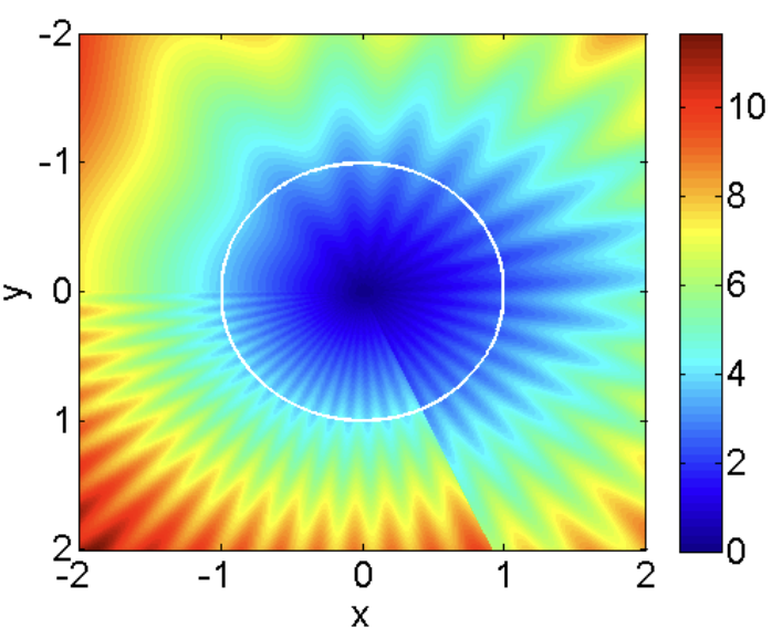
Heatmap of a operate that’s star-convex however not convex. Credit: (Lee and Valiant, 2016).
The opposite assumption that we’ll make is that the gradients $nabla f_i$ are domestically bounded. This assumption is glad by many goals of curiosity, together with least-squares and logistic regression. With this, right here is the primary results of this publish.
Assume that for all $i$, $f_i$ is star-convex round a minimizer $x_star$. Moreover, we’ll additionally assume that the subgradients are bounded within the ball $mathcal{B}$ with middle $x_star$ and radius $|x_0 – x_star|$, that’s, we now have $|nabla f_i(x)|leq G$ for all $i$ and $x in mathcal{B}$. Then, SGD-SPS converges in anticipated operate error at a price of at the least $O(1/sqrt{T})$. That’s, after $T$ steps we now have
start{equation}
min_{t=0, ldots, T-1} ,EE f(x_t) – f(x_star) leq frac{G}{sqrt{T}}|x_0 – x_star| ,.
finish{equation}
The proof principally follows that of Garrigos et al. 2023,
I’ve structured the proof into three elements. 1️⃣ first we’ll set up that the iterates are bounded. It will permit us to keep away from making a worldwide Lipschitz assumption. 2️⃣ then we’ll derive a key inequality that relates the error at two subsequent iterations. In 3️⃣ we’ll sum this inequality over iterations, some phrases will cancel out, and we’ll get the specified convergence price.
1️⃣ Error is monotonically reducing. We would like to indicate that the iterate error $|x_t – x_star|^2$ is monotonically reducing in $t$. Let’s contemplate first the case $|nabla f_i(x_t)| neq 0$, the place $i$ denotes the random index chosen at iteration $t$.
Then utilizing the definition of $x_{t+1}$ and increasing the sq. we now have
start{align}
&|x_{t+1} – x_star|^2 = |x_t – x_star|^2 – 2 stepsize_t langle nabla f_i(x_t), x_t – x_starrangle + stepsize_t^2 |nabla f_i(x_t)|^2 nonumber
&quadstackrel{textual content{(star convexity)}}{leq} |x_t – x_star|^2 – 2 stepsize_t (f_i(x_t) – f_i(x_star)) + stepsize_t^2 |nabla f_i(x_t)|^2 nonumber
&quadstackrel{textual content{(definition of $stepsize_t$)}}{=} |x_t – x_star|^2 – frac{(f_i(x_t) – f_i(x_star))_+^2}^2 label{eq:last_decreasing}
finish{align}
This final equation exhibits that the error is monotonically reducing at any time when $|nabla f_i(x_t)| neq 0$.
Let’s now contemplate the case $|nabla f_i(x_t)| = 0$. On this case, the step-size is 0 by our definition of $stepsize_t$, and so the error is fixed. We’ve established that the error is monotonically reducing in each circumstances.
2️⃣ Key recursive inequality. Let’s once more first contemplate the case $|nabla f_i(x_t)| neq 0$. Since we have established that the error is monotonically reducing, the iterates stay within the ball centered at $x_star$ with radius $|x_0 – x_star|$. We are able to then use the domestically bounded gradients assumption on eqref{eq:last_decreasing} to acquire
start{equation}label{eq:recursive_G}
|x_{t+1} – x_star|^2 leq |x_t – x_star|^2 – frac{1}{G^2}(f_i(x_t) – f_i(x_star))_+^2 ,.
finish{equation}
Let’s now contemplate the case by which $|nabla f_i(x_t)| = 0$. On this case, due to star-convexity, we now have $f_i(x_t) – f_i(x_star) leq 0$ and so $(f_i(x_t) – f_i(x_star))_+ = 0$. Therefore inequality eqref{eq:recursive_G} can also be trivially verified. We’ve established that eqref{eq:recursive_G} holds in all circumstances.
Let $EE_t$ denote the expectation conditioned on all randomness as much as iteration $t$. Then
taking expectations on each side of the earlier inequality and utilizing Jensen’s inequality on the convex operate $z mapsto z^2_{+}$ we now have
start{align}
EE_t|x_{t+1} – x_star|^2 &leq |x_t – x_star|^2 – frac{1}{G^2} EE_t(f_i(x_t) – f_i(x_star))_+^2
&stackrel{mathclap{textual content{(Jensen’s)}}}{leq} |x_t – x_star|^2 – frac{1}{G^2} (f(x_t) – f(x_star))^2 ,,
finish{align}
the place we now have dropped the optimistic half within the final time period, which is non-negative by definition of $x_star$.
Lastly, taking full expectations on each side, utilizing the tower property of expectation and rearranging we now have our key recursive inequality:
start{equation}label{eq:key_inequality}
boxed{vphantom{sum_a^b} EE(f(x_t) – f(x_star))^2 leq G^2(EE|x_t – x_star|^2 – EE|x_{t+1} – x_star|^2)}
finish{equation}
3️⃣ Telescoping and closing price. Utilizing Jensen’s inequality as soon as extra, we now have
start{align}
min_{t=0, ldots, T-1},(EE f(x_t) – f(x_star))^2~&stackrel{mathclap{textual content{(Jensen’s)}}}{leq}~min_{t=0, ldots, T-1} EE(f(x_t) – f(x_star))^2
&leq frac{1}{T}sum_{t=0}^{T-1} EE(f(x_t) – f(x_star))^2
&stackrel{eqref{eq:key_inequality}}{leq} frac{G^2}{T} |x_0 – x_star|^2
finish{align}
Taking sq. roots on each side offers
start{equation}
sqrt{min_{t=0, ldots, T-1},(EE f(x_t) – f(x_star))^2} leq frac{G}{sqrt{T}} |x_0 – x_star|,.
finish{equation}
Lastly, by the monotonicity of the sq. root, we are able to convey the sq. root contained in the $min$ to acquire the specified end result.
Citing
In case you discover this weblog publish helpful, please contemplate citing as
Stochastic Polyak Step-size, a easy step-size tuner with optimum charges, Fabian Pedregosa, 2023
with bibtex entry:
    @misc{pedregosa2023sps,
      title={Stochastic Polyak Step-size, a easy step-size tuner with optimum charges},
      writer={Fabian Pedregosa},
      howpublished = {url{http://fa.bianp.web/weblog/2023/sps/}},
      yr={2023}
    }
Acknowledgments
Because of Robert Gower for first bringing this proof to my consideration, after which for answering all my questions on it. Thanks additionally to Vincent Roulet for proof studying this publish and making many helpful options.
References
[ad_2]