This text was initially revealed by Ampere Computing.

I noticed a weblog put up about gprofng, a brand new GNU profiling software. The instance in that weblog was a matrix-vector multiplication program written in C. I’m a Java™ programmer, and profiling Java functions is typically troublesome with instruments which can be designed for statically-compiled C packages, quite than Java packages which can be compiled at runtime. On this weblog I present that gprofng is straightforward to make use of and helpful for digging into the dynamic conduct of a Java software.

Step one was to write down a matrix multiplication program. I wrote a full matrix-times-matrix program as a result of it’s not tougher than matrix-times-vector. There are three principal strategies: one technique to compute the inner-most multiply-add, one technique to mix multiply-adds right into a single ingredient of the consequence, and one technique to iterate computing every ingredient of the consequence.

I wrapped the computation in a easy harness to compute the matrix product repeatedly, to ensure the instances are repeatable. (See Finish Notice 1.) This system prints out when every matrix multiplication begins (relative to the beginning of the Java digital machine), and the way lengthy every matrix multiply takes. Right here I ran the check to multiply two 8000×8000 matrices. The harness repeats the computation 11 instances, and to raised spotlight the conduct later, sleeps for 920 milliseconds between the repetitions:

$ numactl --cpunodebind=0 --membind=0 -- 
java -XX:+UseParallelGC -Xms31g -Xmx31g -Xlog:gc -XX:-UsePerfData 
  MxV -m 8000 -n 8000 -r 11 -s 920

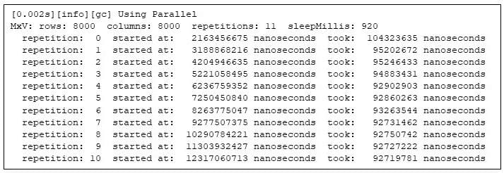
Determine 1: Operating the matrix multiply program

Notice that the second repetition takes 92% of the time of the primary repetition, and the final repetition takes solely 89% of the primary repetition. These variations within the execution instances verify that Java packages want a while to heat up.

The query is: Can I take advantage of gprofng to see what is occurring between the primary repetition and the final repetition that makes the efficiency enhance?

One solution to reply that query is to run this system and let gprofng accumulate details about the run. Happily, that’s simple: I merely prefix the command line with a gprofng command to gather what gprofng calls an “experiment.”:

$ numactl --cpunodebind=0 --membind=0 -- 
gprofng accumulate app 
    java -XX:+UseParallelGC -Xms31g -Xmx31g -Xlog:gc --XX:-UsePerfData 
        MxV -m 8000 -n 8000 -r 11 -s 920

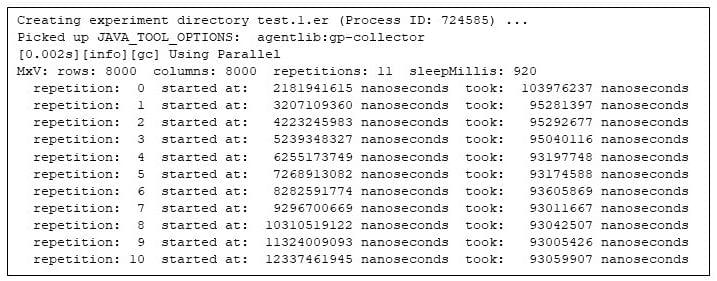
Determine 2: Operating the matrix multiply program underneath gprofng

The very first thing to notice, as with all profiling software, is the overhead that gathering profiling info imposes on the applying. In comparison with the earlier, unprofiled run, gprofng appears to impose no noticeable overhead.

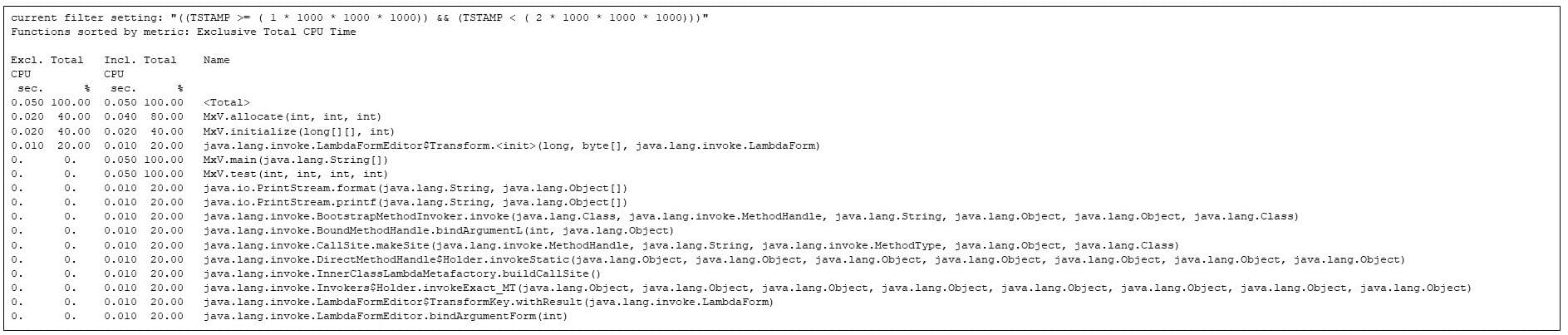
I can then ask gprofng how the time was spent in the complete software. (See Finish Notice 2.) For the entire run, gprofng says the most popular 24 strategies are:

$ gprofng show textual content check.1.er -viewmode skilled -limit 24 -functions

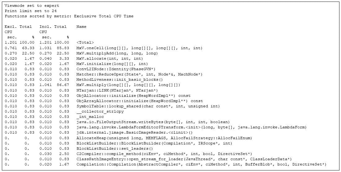
Determine 3: Gprofng show of the most popular 24 strategies

The features view proven above offers the unique and inclusive CPU instances for every technique, each in seconds and as a share of the whole CPU time. The operate named is a pseudo operate generated by gprofng and has the whole worth of the assorted metrics. On this case I see that the whole CPU time spent on the entire software is 1.201 seconds.

The strategies of the applying (the strategies from the category MxV) are in there, taking on the overwhelming majority of the CPU time, however there are another strategies in there, together with the runtime compiler of the JVM (Compilation::Compilation), and different features that aren’t a part of the matrix multiplier. This show of the entire program execution captures the allocation (MxV.allocate) and initialization (MxV.initialize) code, which I’m much less curious about since they’re a part of the check harness, are solely used throughout start-up, and have little to do with matrix multiplication.

I can use gprofng to concentrate on the components of the applying that I’m curious about. One of many fantastic options of gprofng is that after gathering an experiment, I can apply filters to the gathered knowledge. For instance, to have a look at what was taking place throughout a specific interval of time, or whereas a specific technique is on the decision stack. For demonstration functions and to make the filtering simpler, I added strategic calls to Thread.sleep(ms) in order that it could be simpler to write down filters based mostly on program phases separated by one-second intervals. That’s the reason this system output above in Determine 1 has every repetition separated by about one second though every matrix a number of takes solely about 0.1 seconds.

gprofng is scriptable, so I wrote a script to extract particular person seconds from the gprofng experiment. The primary second is all about Java digital machine startup.

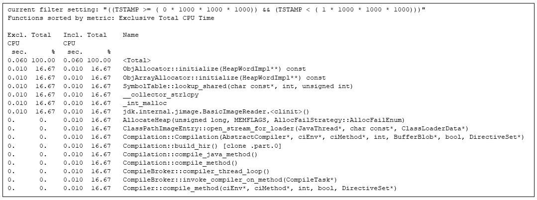
Determine 4: Filtering the most popular strategies within the first second. The matrix multiply has been artificially delayed throughout this second to permit me to point out the JVM to start out up

I can see that the runtime compiler is kicking in (e.g., Compilation::compile_java_method, taking 16% of the CPU time), though not one of the strategies from the applying has begun operating. (The matrix multiplication calls are delayed by the sleep calls I inserted.)

After the primary second is a second throughout which the allocation and initialization strategies run, together with varied JVM strategies, however not one of the matrix multiply code has began but.

Determine 5: The most well liked strategies within the second second. The matrix allocation and initialization is competing with JVM startup

Now that JVM startup and the allocation and initialization of the arrays is completed, the third second has the primary repetition of the matrix multiply code, proven in Determine 6. However word that the matrix multiply code is competing for machine sources with the Java runtime compiler (e.g., CompileBroker::invoke_compiler_on_method, 8% in Determine 6), which is compiling strategies because the matrix multiply code is discovered to be sizzling.

Even so, the matrix multiplication code (e.g., the “inclusive” time within the MxV.predominant technique, 91%) is getting the majority of the CPU time. The inclusive time says {that a} matrix multiply (e.g., MxV.multiply) is taking 0.100 CPU seconds, which agrees with the wall time reported by the applying in Determine 2. (Gathering and reporting the wall time takes some wall time, which is exterior the CPU time gprofng accounts to MxV.multiply.)

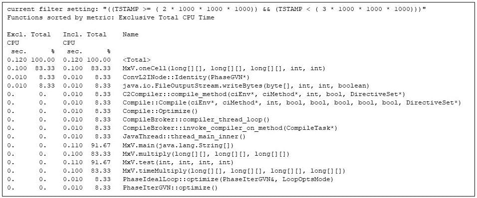
Determine 6: The most well liked strategies within the third second, displaying that the runtime compiler is competing with the matrix multiply strategies

On this explicit instance the matrix multiply will not be actually competing for CPU time, as a result of the check is operating on a multi-processor system with loads of idle cycles and the runtime compiler runs as separate threads. In a extra constrained circumstances, for instance on a heavily-loaded shared machine, that 8% of the time spent within the runtime compiler could be a difficulty. Then again, time spent within the runtime compiler produces extra environment friendly implementations of the strategies, so if I had been computing many matrix multiplies that’s an funding I’m keen to make.

By the fifth second the matrix multiply code has the Java digital machine to itself.

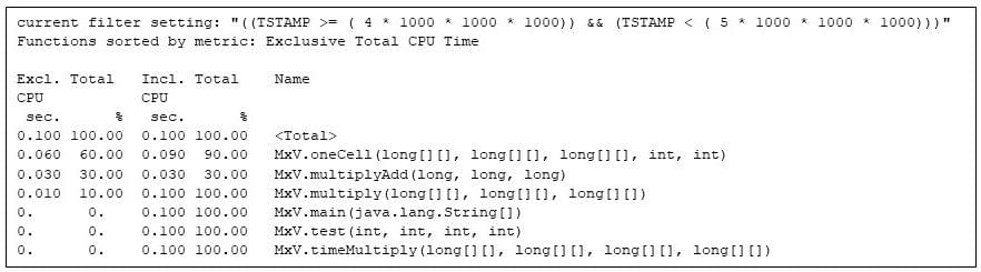
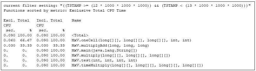
Determine 7: All of the operating strategies in the course of the fifth second, displaying that solely the matrix multiply strategies are energetic

Notice the 60%/30%/10% cut up in unique CPU seconds between MxV.oneCell, MxV.multiplyAdd, and MxV.multiply. The MxV.multiplyAdd technique merely computes a multiply and an addition: however it’s the innermost technique within the matrix multiply. MxV.oneCell has a loop that calls MxV.multiplyAdd. I can see that the loop overhead and the decision (evaluating conditionals and transfers of management) are comparatively extra work than the straight arithmetic in MxV.multiplyAdd. (This distinction is mirrored within the unique time for MxV.oneCell at 0.060 CPU seconds, in comparison with 0.030 CPU seconds for MxV.multiplyAdd.) The outer loop in MxV.multiply executes sometimes sufficient that the runtime compiler has not but compiled it, however that technique is utilizing 0.010 CPU seconds.

Matrix multiplies proceed till the ninth second, when the JVM runtime compiler kicks in once more, having found that MxV.multiply has grow to be sizzling.

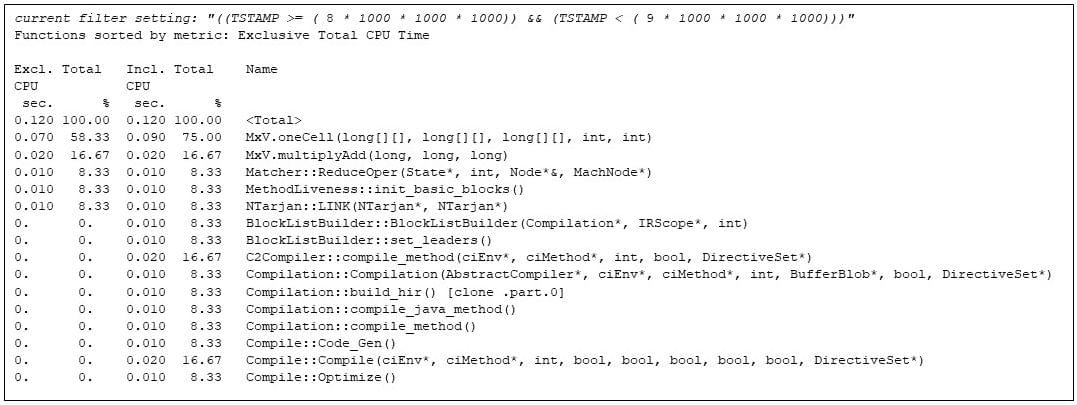
By the ultimate repetition, the matrix multiplication code has full use of the Java digital machine.

Determine 9: The ultimate repetition of the matrix multiply program, displaying the ultimate configuration of the code

Conclusion

I’ve proven how simple it’s to achieve perception into the runtime of Java functions by profiling with gprofng. Utilizing the filtering function of gprofng to look at an experiment by time slices allowed me to look at simply this system phases of curiosity. For instance, excluding allocation and initialization phases of the applying, and displaying only one repetition of this system whereas the runtime compiler is working its magic, which allowed me to spotlight the enhancing efficiency as the new code was progressively compiled.

Additional Studying

For readers who wish to study extra about gprofng, there’s this weblog put up with an introductory video on gprofng, together with directions on set up it on Oracle Linux.

Acknowledgements

Due to Ruud van der Pas, Kurt Goebel, and Vladimir Mezentsev for ideas and technical assist, and to Elena Zannoni, David Banman, Craig Hardy, and Dave Neary for encouraging me to write down this weblog.

Finish Notes

1. The motivations for the parts of this system command line are:

• numactl --cpunodebind=0 --membind=0 --. Prohibit the reminiscence utilized by the Java digital machine to cores and reminiscence of 1 NUMA node. Limiting the JVM to at least one node reduces run-to-run variation of this system.
• java. I’m utilizing OpenJDK construct of jdk-17.0.4.1 for aarch64.
• -XX:+UseParallelGC. Allow the parallel rubbish collector, as a result of it does the least background work of the accessible collectors.
• -Xms31g -Xmx31g. Present ample Java object heap area to by no means want a rubbish assortment.
• -Xlog:gc. Log the GC exercise to confirm {that a} assortment is certainly not wanted. (“Belief however confirm.”)
• -XX: -UsePerfData. Decrease the Java digital machine overhead.

2. The reasons of the gprofng choices are:

• -limit 24. Present solely the highest 24 strategies (right here sorted by unique CPU time). I can see that the show of 24 strategies will get me properly down into the strategies that use virtually no time. Later I’ll use restrict 16 in locations the place 16 strategies get all the way down to the strategies that contribute insignificant quantities of CPU time. In a number of the examples, gprofng itself limits the show, as a result of there will not be that many strategies that accumulate time.
• -viewmode skilled. Present all of the strategies that accumulate CPU time, not simply Java strategies, together with strategies which can be native to the JVM itself. Utilizing this flag permits me to see the runtime compiler strategies, and so on.